Approximating Standard Deviation from Inter-Quantile Range

Occasionally researchers report inter-quantile ranges (e.g., inter-quartile range) to measure the spread of the data. Since meta-analysts need standard deviations to calculate effect size estimates, here is a strategy to approximate them from an inter-quantile range.

Inter-Quantile Range

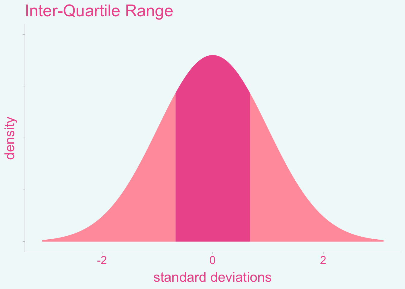
Studies may report inter-quantile ranges in order to communicate the spread of the data. However, meta-analysts will need standard deviations (SD) to calculate effect size estimates such as standardized mean differences (i.e., Cohen’s $d$). For this post, we will focus on the inter-quartile range (IQR) although the method described here will apply to any range between a pair of quantiles. The IQR ($X_{(75-25)}$) is defined as the difference between the 75th and 25th quantile values, that is, the region where 50% of the data lies. We can visualize what this will look like with normally distributed data:

Now let’s compare the range of values covered by +/- 1 SDs of a normal distribution:

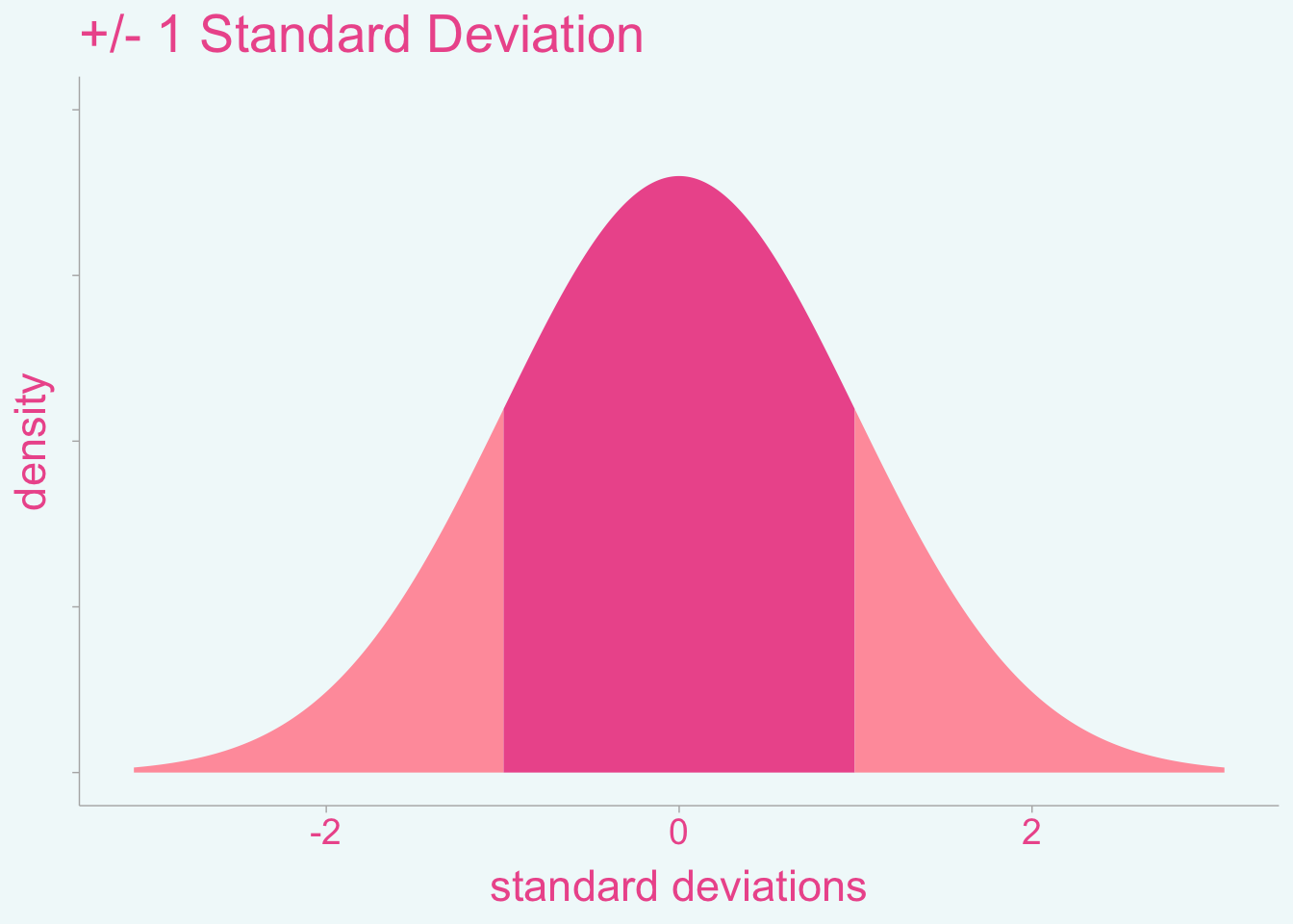
The range covered by $\pm 1$ SD covers a considerably larger range of values than the IQR.

Step 2: Convert IQR to Standard Deviations

The quantile function (${\varphi }^{-1}$) of the standard normal distribution (i.e., mean=0, SD=1) converts quantiles of the cumulative density function into the corresponding values in standard deviation units. The difference between the corresponding values will give us the IQR in SD units,

$$S_{(75-25)}={\varphi }^{-1}(.75)-{\varphi }^{-1}(.25)$$ The resulting value is $S_{(75-25)}=1.34898$. It is important to note that this formulation can be used for any set of quantiles not just IQR, therefore we can generalized this to compare any arbitrary pair of quantiles ($Q1,Q2$),

$$S_{(Q_2-Q_1)}={\varphi }^{-1}(Q_2)-{\varphi }^{-1}(Q_1)$$

Now that we have the IQR in terms of SD units, we can divide with the raw IQR to obtain an estimate of the SD of $X$ ($S_X$),

$$S_X=\frac{X_{(75-25)}}{S_{(75-25)}}=\frac{X_{(75-25)}}{1.34898}$$

# Define IQR
X_25 <- 30
X_75 <- 50
X_75_25 <- X_75 - X_25

# Compute IQR in SDs
S_75_25 <- qnorm(.75) - qnorm(.25)

# Estimate standard deviation
S_X <-  X_75_25 / S_75_25

#print results
print(S_X)

[1] 14.82602

Note the Assumptions!

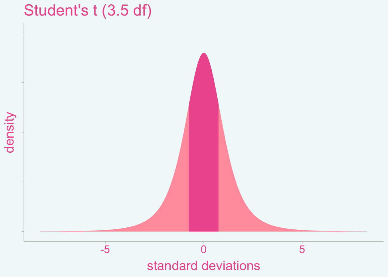
Since this method provides an approximation of a normal distribution it is important to point out that the method may be biased under different distributions. For example, if we try the same method on a Student’s t distribution with heavy tails (3.5 degrees of freedom), $S_{(75-25)}$ would be equal to 1.50187 which is slightly larger than 1.34898 that we computed from the normal distribution. If we were to assume a normal distribution when it was truly a student’s t, the method would over-estimate the standard deviation by ~11%.

Applying it to simulated data

Lets see how it performs in simulated sample of normally distributed data… Close enough!!

# Set seed
set.seed(343)

# Simulate normal data (Mean = 10, SD = 5)
X = rnorm(100,10,5)

# Define IQR
q25 <- as.numeric(quantile(X,.25))
q75 <- as.numeric(quantile(X,.75))
X_75_25 <- q75 - q25

# Compute IQR in SD units
S_75_25 <- qnorm(.75) - qnorm(.25)

# Estimate standard deviation
S_X <-  X_75_25 / S_75_25

# Print results
print(S_X)

[1] 4.706901